Transformer Architecture in Deep Learning
Transformers are the architecture behind most modern large language models, many advanced vision systems, multimodal models, code-generation systems, speech models, and an expanding range of scientific AI applications.
Their influence can make the architecture appear almost mystical. It is not. A Transformer is ultimately a carefully arranged collection of matrix multiplications, normalization operations, nonlinear transformations, and attention mechanisms. None of these components is individually magical. The remarkable capability emerges from how they are combined, repeated at scale, and trained on large amounts of data.
The central idea is deceptively simple:
Instead of processing a sequence strictly one element at a time, allow every element to examine the other relevant elements and construct a context-aware representation of itself.
For a sentence, this means that the representation of a word such as “bank” can change depending on whether nearby words include river, loan, money, or fishing. For an image, one patch can examine other image patches. For audio, one time segment can relate itself to distant segments. The architecture does not fundamentally insist that its input must be language; it mainly expects a sequence of representable units.
This article begins with the problems that preceded the Transformer, examines every major architectural component, and then follows information through a Transformer step by step—from raw input to output probabilities.
1. Deep Learning
Deep learning is a subset of machine learning driven by multilayered neural networks whose design is inspired by the structure of the human brain. Rather than depending primarily on hand-crafted rules or manually engineered features, deep learning systems learn useful representations directly from data by adjusting millions or even billions of parameters during training.
Its defining idea is depth. A shallow model may capture only limited patterns, but a deep network stacks many layers so that simple signals can be progressively transformed into richer abstractions. In image tasks, early layers may detect edges and textures before later layers capture shapes and objects. In language tasks, early layers may encode token-level patterns before deeper layers model syntax, semantics, and longer-range relationships.
This layered learning process is what made modern breakthroughs possible across vision, speech, natural language processing, recommendation systems, and scientific modelling. Deep learning works especially well when three conditions align: large training datasets, substantial compute, and architectures capable of learning complex nonlinear relationships.
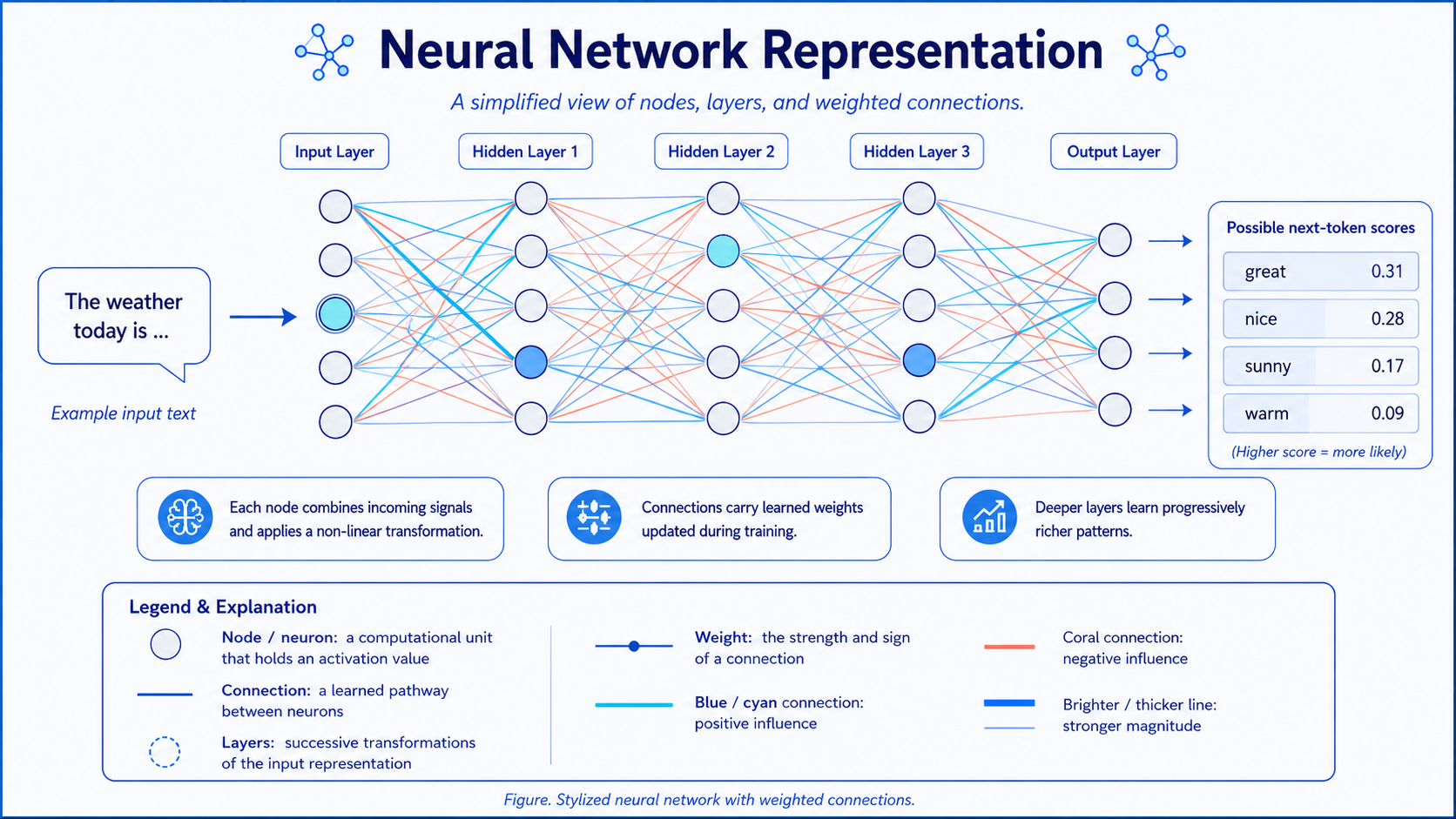
The diagram shows the basic anatomy of a neural network. Input nodes receive raw features, each connection carries a learnable weight, and hidden layers repeatedly transform the signal through weighted sums and activation functions. As information moves forward, the network builds more expressive internal representations. The output layer then turns those learned representations into a decision, score, class, or probability distribution depending on the task.
Transformers sit squarely inside this deep learning landscape. They are not separate from neural networks; they are a modern neural-network architecture built for sequence and structured data. What distinguishes them is that they organize representation learning around attention rather than relying primarily on recurrence. With that grounding in deep learning, we can now look directly at what a Transformer is and why its design mattered so much.
2. What Is a Transformer?
A Transformer is a neural-network architecture designed to model relationships within sequential or structured data. Its defining mechanism is attention, particularly self-attention, which allows each element in a sequence to determine how strongly it should incorporate information from other elements.
The original Transformer introduced in the 2017 paper Attention Is All You Need was designed for machine translation. It contained two major systems:
- An encoder, which processed and represented the input sequence.
- A decoder, which generated the output sequence while consulting the encoder.
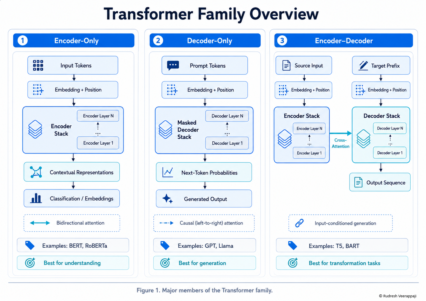
The architecture avoided the recurrent processing used by earlier sequence models. Instead of reading a sentence through a single sequential chain, it could process many positions in parallel during training. This made the model more compatible with highly parallel computing hardware and created shorter computational paths between distant elements in a sequence. Models frequently use only part of this original design:
| Architecture | Primary purpose | Typical examples |
|---|---|---|
| Encoder-only | Understanding and representing input | BERT-style models, classifiers, embedding models |
| Decoder-only | Autoregressive generation | GPT-style language models |
| Encoder–decoder | Transforming one sequence into another | T5-style models, translation and summarization systems |
These are not three unrelated inventions. They are different arrangements of the same architectural family.
A useful first mental model
Imagine a Transformer as a conference attended by tokens.
Each token arrives with:
- an identity,
- a numerical representation,
- and information about where it appeared.
During self-attention, each token consults the other tokens and asks:
“Which of you are relevant to what I currently mean?”
After that discussion, every token independently passes through a small neural network to refine what it has learned. This process repeats across many layers. By the final layer, the tokens no longer contain merely dictionary-like meanings; they contain context-dependent representations shaped by the entire sequence available to them.
The conference analogy is imperfect, but it is considerably better than imagining words travelling down a single-file queue while carrying increasingly overworked suitcases of context.
3. Why Was the Transformer Needed?
Understanding the Transformer is easier when we understand the architectural frustrations that preceded it.
3.1 Sequence modelling before Transformers
Language, audio, financial time series, biological sequences, and many other forms of data have an ordering. The meaning of an element often depends on elements that appeared earlier or later.
For example:
“The application failed because the database connection had expired.”
The meaning of expired depends on its relationship with database connection. A useful sequence model must preserve such relationships even when the related elements are far apart.
Earlier neural sequence models primarily used Recurrent Neural Networks, or RNNs. An RNN processes a sequence one step at a time:
Token 1 → Hidden state 1
Token 2 + Hidden state 1 → Hidden state 2
Token 3 + Hidden state 2 → Hidden state 3
...
The hidden state acts as a running memory. In theory, it can carry information from the beginning of a sequence to the end. In practice, long sequences create optimization difficulties, including vanishing or exploding gradients and the gradual dilution of earlier information.
Long Short-Term Memory networks, or LSTMs, and Gated Recurrent Units, or GRUs, introduced gating mechanisms that improved memory retention. Sequence-to-sequence systems subsequently used one recurrent network to encode an input and another to decode an output. This arrangement worked, but it created two important constraints.
Constraint 1: Sequential computation
An RNN generally cannot calculate the state for token 20 before calculating the state for token 19. The computation therefore resembles a relay race: no matter how many processors are available, the baton must still be passed in sequence.
Constraint 2: Information bottlenecks
Early encoder–decoder systems compressed an entire input sequence into a fixed-length vector. Asking one vector to preserve every relevant detail of a long paragraph is rather like asking someone to summarize an entire technical meeting on a single sticky note—and then translate it accurately.
3.2 Attention begins solving the bottleneck
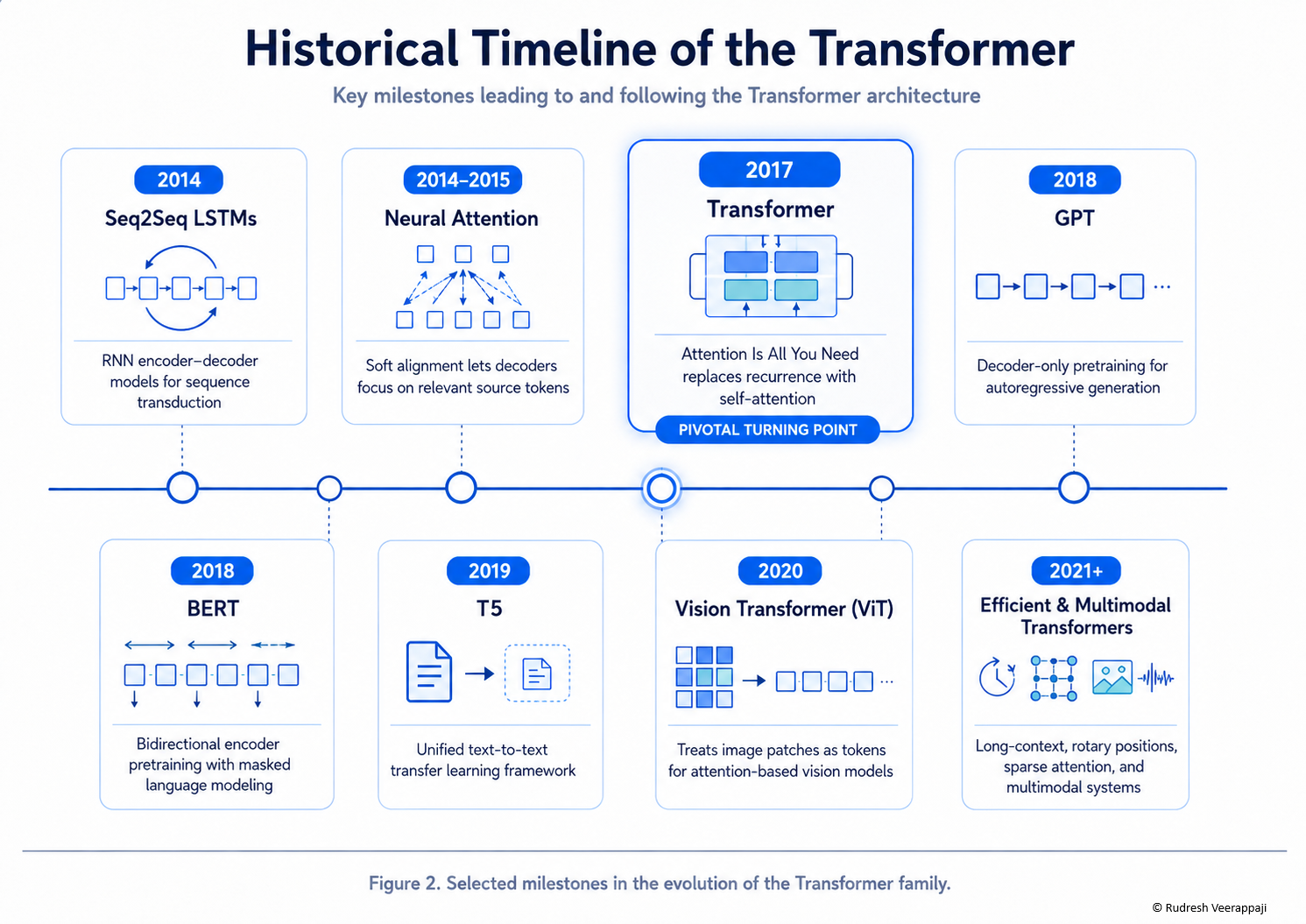
In 2014, Bahdanau, Cho, and Bengio proposed an attention-based neural machine-translation system. Rather than forcing the decoder to rely exclusively on one fixed representation, the decoder could examine different encoder states while producing each output word.
When translating a particular target word, the model learned to assign higher importance to the relevant source words. This created a soft, learned alignment between the input and output sequences. Attention was therefore present before the Transformer. The Transformer’s decisive move was more radical:
Remove recurrence as the primary mechanism and build the architecture around attention itself.
3.3 The 2017 Transformer
In June 2017, researchers introduced the Transformer in Attention Is All You Need. The architecture used stacked attention and feed-forward layers for both its encoder and decoder, eliminating recurrent and convolutional sequence processing from the central architecture. It offered several important advantages:
- sequence positions could be processed in parallel during training;
- every token could establish a relatively direct relationship with every other visible token;
- the architecture mapped efficiently onto GPUs and other matrix-processing hardware;
- the same basic block could be stacked repeatedly;
- the architecture was flexible enough to be adapted beyond translation.
3.4 What followed
The years after 2017 demonstrated that Transformer blocks could support several different learning objectives.
- GPT-style models showed how decoder-based Transformers could be pretrained through autoregressive next-token prediction.
- BERT used an encoder-based Transformer to learn bidirectional representations from masked text.
- T5 treated many language tasks as text-to-text transformations using an encoder–decoder architecture.
- Vision Transformer, or ViT, represented an image as a sequence of patches and processed them using a Transformer encoder.
These developments helped establish the Transformer not simply as an NLP architecture, but as a general method for learning relationships among elements in structured data.
Further Reading
- Sutskever, Vinyals and Le — Sequence to Sequence Learning with Neural Networks
- Bahdanau, Cho and Bengio — Neural Machine Translation by Jointly Learning to Align and Translate
- Vaswani et al. — Attention Is All You Need
4. The Transformer at a Glance
Before examining the individual components, it is useful to see the full data path.
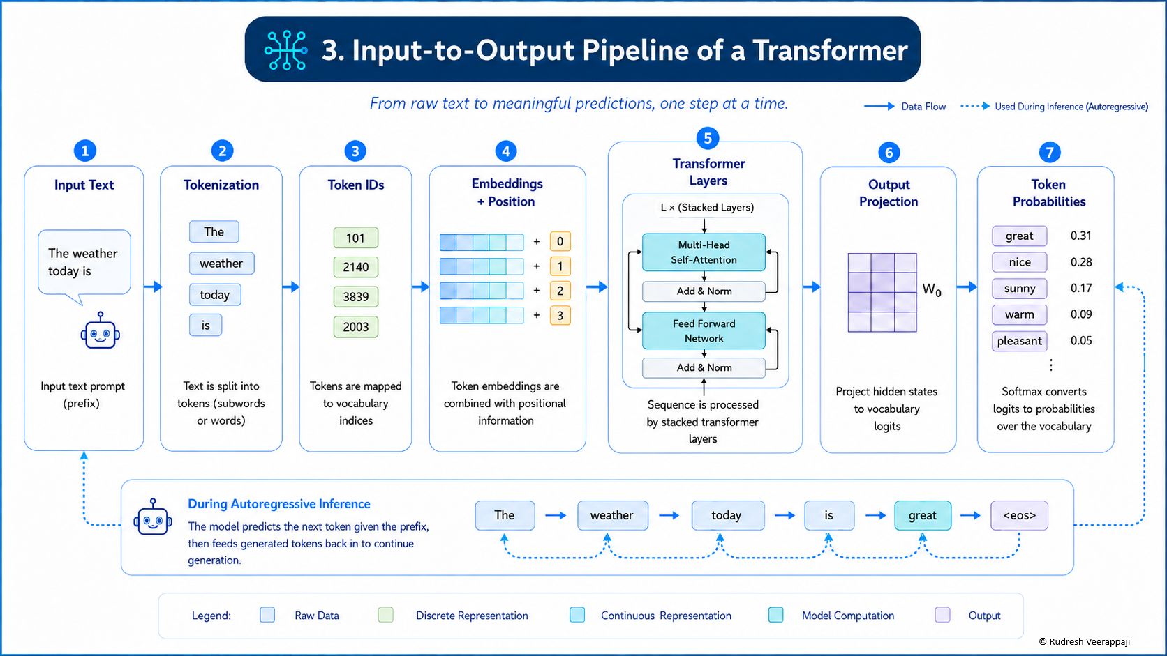
For a text-based Transformer, the general pipeline is:
Raw text
   ↓
Tokenization
   ↓
Token IDs
   ↓
Token embeddings
   +
Positional information
   ↓
Transformer blocks
   ├── Attention
   ├── Residual connection
   ├── Normalization
   ├── Feed-forward network
   └── Residual connection and normalization
   ↓
Contextual representations
   ↓
Task-specific output layer
   ↓
Probabilities, embeddings or predictions
A decoder-only language model uses this process to estimate the probability distribution of the next token. An encoder-only model may produce a classification or an embedding. An encoder–decoder model represents an input and then generates a corresponding output sequence.
The important point is that the Transformer block does not directly receive ordinary words. It receives tensors: multidimensional arrays of numbers.
Step 5.1: Tokenization
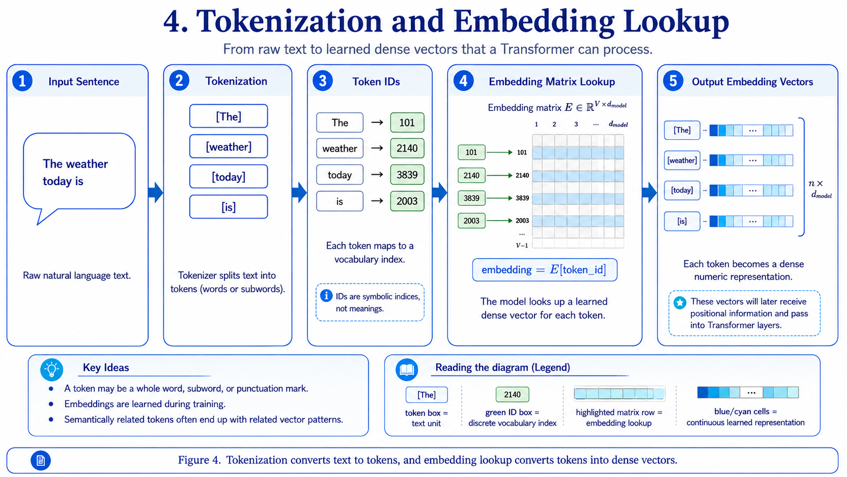
Neural networks operate on numbers, not raw strings. Before text enters a Transformer, a tokenizer divides it into units called tokens and maps each token to an integer identifier.
Consider:
Transformers understand context.
A tokenizer might divide this into something resembling:
["Transform", "ers", " understand", " context", "."]
Another tokenizer could produce a different segmentation. Tokens are not necessarily complete words. They may represent:
- whole words,
- parts of words,
- punctuation,
- whitespace patterns,
- individual characters,
- bytes,
- or combinations of these.
This subword approach allows the system to represent rare or previously unseen words using reusable pieces. For example, a tokenizer may decompose uncharacteristically into several familiar subword units rather than requiring one dedicated vocabulary entry.
SentencePiece is one influential tokenization system that can train subword models directly from raw text without requiring language-specific pre-tokenization. n IDs
Each token corresponds to an integer in the model’s vocabulary:
"Transform"  →  18342
"ers"        →  719
" understand"→  3612
"context"    →  4967
"."          →  13
These numbers are identifiers, not semantic quantities. Token 18,342 is not inherently “more Transformer-like” than token 719. The IDs are closer to catalogue numbers than measurements.
A technical clarification
Tokenization is essential to the language-model pipeline, but it is not mathematically part of the Transformer block itself. The tokenizer is the reception desk. It issues the badges; it does not attend the meeting.
Further Reading
- Kudo and Richardson — SentencePiece: A Simple and Language Independent Subword Tokenizer and Detokenizer
- Hugging Face documentation — Tokenizers and subword processing
Step 5.2: Token Embeddings
Token IDs are discrete symbols. Neural networks need continuous numerical representations that can be adjusted through gradient-based learning.
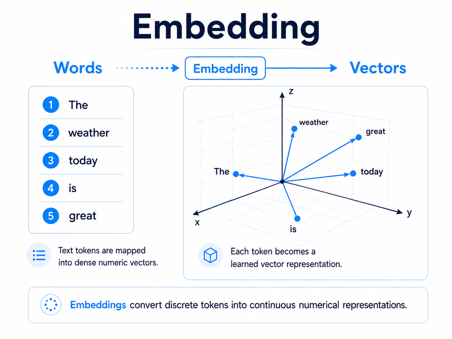
An embedding layer contains a trainable matrix:
E \in \mathbb{R}^{V \times d_{\text{model}}}
where:
- (V) is the vocabulary size;
- (d_{\text{model}}) is the dimensionality of the model’s internal representation.
Looking up a token ID selects one row of this matrix.
If:
- the vocabulary contains 50,000 tokens;
- the model dimension is 768;
then the embedding matrix has the shape:
50{,}000 \times 768
Every token becomes a vector containing 768 learned values.
For a sequence containing (n) tokens, the embedding output has the shape:
X \in \mathbb{R}^{n \times d_{\text{model}}}
The model therefore retains one vector per token. It does not immediately add every word together into one sentence vector. Doing that would destroy much of the sequence structure before the interesting work had even begun.
Static identity versus contextual meaning
At the embedding stage, the token bank begins with the same learned base vector in both sentences:
“The canoe reached the bank.”
“The bank approved the loan.”
The surrounding context has not yet been fully incorporated. Attention layers progressively modify the representation, causing the final contextual vector for bank to differ across the two sentences.
The embedding says roughly, “This token is bank.”
The Transformer layers add, “In this particular sentence, this instance of bank refers to the side of a river.”
Google’s machine-learning documentation describes embeddings as dense vector representations whose values are learned during training, enabling related items to acquire useful geometric relationships.
Step 5.3: Positional Information
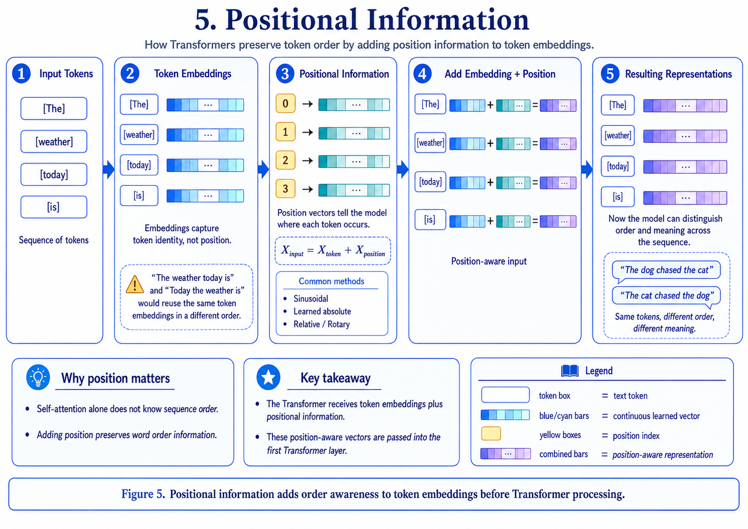
Self-attention does not process tokens through a recurrent chain. By itself, the basic attention calculation has no inherent understanding that one token came before another.
Without positional information, these sequences would contain the same token identities:
The dog chased the cat.
The cat chased the dog.
Humans notice a fairly significant difference. The dog and cat certainly would.
The model must therefore receive information about token order.
5.3.1 Sinusoidal positional encoding
The original Transformer added deterministic sinusoidal positional vectors to token embeddings. Different dimensions used sine and cosine functions with different frequencies:
PE(pos,2i)=\sin\left(\frac{pos}{10000^{2i/d_{\text{model}}}}\right)
PE(pos,2i+1)=\cos\left(\frac{pos}{10000^{2i/d_{\text{model}}}}\right)
Here:
- (pos) is the token position;
- (i) identifies a dimension within the positional vector.
The input to the first Transformer layer becomes:
X_{\text{input}} = X_{\text{token}} + X_{\text{position}}
The resulting vector communicates both token identity and location.
5.3.2 Learned positional embeddings
Instead of fixed sinusoidal functions, some models learn a positional vector for each supported position. Position 1 has a trainable vector, position 2 has another, and so forth.
This is straightforward but can make extrapolation beyond the trained position range difficult.
5.3.3 Relative and rotary position methods
Many later architectures represent relative distance or integrate position directly into the attention calculation. Rotary Position Embedding, or RoPE, rotates query and key vectors according to their positions, allowing relative positional relationships to influence attention scores. The specific mechanism varies by model, but its purpose remains consistent:
Tell the architecture not only what the tokens are, but where they are and how far apart they occur.
Further Reading
- Vaswani et al. — Section 3.5 of Attention Is All You Need
- Su et al. — RoFormer: Enhanced Transformer with Rotary Position Embedding
Step 5.4: Self-Attention
Self-attention is the central mechanism of the architecture.
Its purpose is to calculate a new representation for each token by combining information from the tokens that are relevant to it.
Consider:
“The satellite transmitted the measurements after it entered orbit.”
To construct a useful representation for it, the model should connect the pronoun strongly with satellite. To interpret measurements, it may attend to transmitted. To understand orbit, it may relate it to satellite and entered.
Self-attention provides a learned procedure for constructing these relationships.
5.4.1 Queries, keys and values
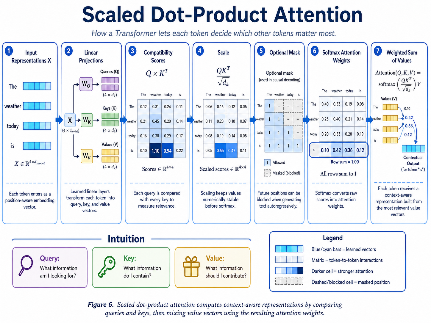
Each input vector is transformed into three vectors:
- a query;
- a key;
- a value.
For input matrix (X):
Q=XW_Q
K=XW_K
V=XW_V
The matrices (W_Q), (W_K), and (W_V) are learned during training.
A useful analogy is a technical knowledge base:
- Query: What information am I looking for?
- Key: What kind of information does this item contain?
- Value: What information should be returned if this item is relevant?
For the token it, the query may seek an earlier noun that could act as its referent. The key produced by satellite may match that query strongly. The corresponding value then contributes heavily to the new representation of it.
The labels query, key and value come from retrieval systems, but in a Transformer they are all learned projections of the current token representations.
5.4.2 Calculating compatibility scores
A query is compared with every visible key using a dot product:
QK^T
If there are (n) tokens, this produces an (n \times n) score matrix.
Each row answers:
For this querying token, how relevant is every token in the sequence?
A high dot product indicates that the query and key point in compatible directions in the learned vector space.
5.4.3 Why the scores are scaled
The raw dot products are divided by the square root of the key dimension:
\frac{QK^T}{\sqrt{d_k}}
As (d_k) grows, unscaled dot products can become large in magnitude. Large values can push the softmax function into regions with extremely concentrated probabilities and very small gradients. Scaling helps keep the score distribution numerically manageable.
5.4.4 Applying the softmax function
Softmax converts each row of scores into non-negative weights that sum to one:
A=\operatorname{softmax}\left(\frac{QK^T}{\sqrt{d_k}}\right)
If the attention weights for one token are:
satellite       0.64
transmitted     0.08
measurements    0.05
after           0.02
it              0.11
entered         0.06
orbit           0.04
then satellite contributes most strongly to that token’s updated representation.
These numbers are only illustrative. The actual model learns its own attention patterns.
5.4.5 Combining the values
The attention weights are multiplied by the value vectors:
\operatorname{Attention}(Q,K,V)
===============================

\operatorname{softmax}
\left(
\frac{QK^T}{\sqrt{d_k}}
\right)V
The output for every token is therefore a weighted mixture of the value vectors from relevant positions. This is the standard scaled dot-product attention operation introduced in the original architecture and exposed directly in modern deep-learning frameworks.
Result: contextualized token representations
Before self-attention:
"it" ≈ generic pronoun representation
After self-attention:
"it" ≈ pronoun referring to the satellite in this sentence
The token has not been replaced by another token. Its vector has been enriched with context.
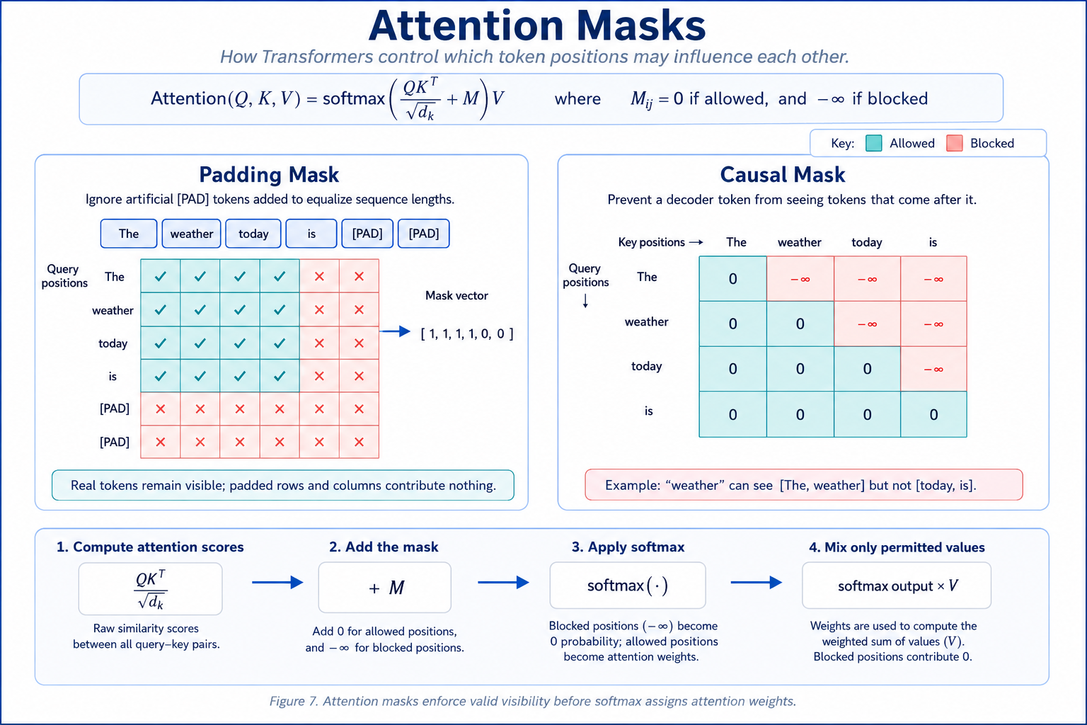
Step 5.5: Attention Masks
Not every token should always be allowed to examine every other token. Transformers use masks to modify which relationships are permitted.
The mask can be incorporated into the attention equation:
\operatorname{Attention}(Q,K,V)
===============================

\operatorname{softmax}
\left(
\frac{QK^T}{\sqrt{d_k}} + M
\right)V
Masked positions receive a very large negative score before softmax, making their resulting attention weights approximately zero.
5.5.1 Padding masks
Sequences in a batch frequently have different lengths. Shorter sequences may be padded to produce uniform tensor dimensions:
Sequence A: [The, model, failed, ., PAD, PAD]
Sequence B: [The, model, completed, the, task, .]
Padding tokens do not represent meaningful content. A padding mask prevents genuine tokens from attending to them.
Without the mask, the model could spend computation studying artificial blanks. That would be the neural-network equivalent of carefully interviewing empty chairs.
5.5.2 Causal masks
Autoregressive decoders predict future tokens from earlier tokens. During training, the full target sentence may be available in memory, but token position (t) must not inspect positions after (t).
A causal mask forms a lower-triangular visibility pattern:
Token 1 can see: 1
Token 2 can see: 1, 2
Token 3 can see: 1, 2, 3
Token 4 can see: 1, 2, 3, 4
For example, when learning to predict:
The spacecraft entered orbit
the representation used to predict orbit may see:
The spacecraft entered
but it must not quietly look at orbit in the answer column and congratulate itself on excellent forecasting.
Causal masking is what makes decoder self-attention masked self-attention.
Step 5.6: Multi-Head Attention
A single attention operation produces one learned pattern of relevance. Language and other structured data, however, contain several relationships at once.
A token may need to track:
- grammatical dependencies;
- nearby modifiers;
- long-distance references;
- entity relationships;
- temporal order;
- topic continuity;
- formatting patterns;
- or task-specific associations.
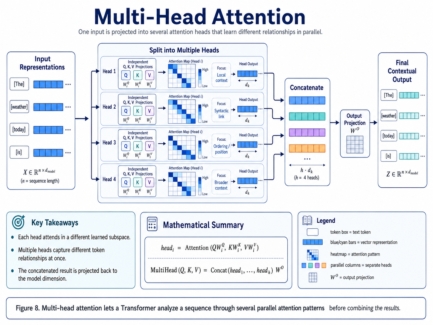
Multi-head attention allows the model to perform several attention operations in parallel.
For attention head (i):
head_i =
\operatorname{Attention}
\left(
QW_i^Q,
KW_i^K,
VW_i^V
\right)
The head outputs are concatenated and projected:
\operatorname{MultiHead}(Q,K,V)
===============================

\operatorname{Concat}
(head_1,\ldots,head_h)W^O
If:
d_{\text{model}}=768
and the model uses 12 heads, each head may use a dimension of:
d_k=64
The heads examine the sequence through different learned projection spaces.
A committee of specialists
One can imagine several reviewers reading the same sentence:
- one focuses on subject–verb relationships;
- one watches pronouns;
- one tracks nearby context;
- one checks long-distance dependencies;
- one notices punctuation or structure.
Their findings are combined before being passed onward.
This is an intuition, not a guarantee that every head develops one clean human-readable function. Learned attention heads can be redundant, distributed, mixed, or difficult to interpret. The committee may contain specialists, generalists, and at least one member whose exact contribution nobody can explain during the meeting.
Step 5.7: Residual Connections and Layer Normalization
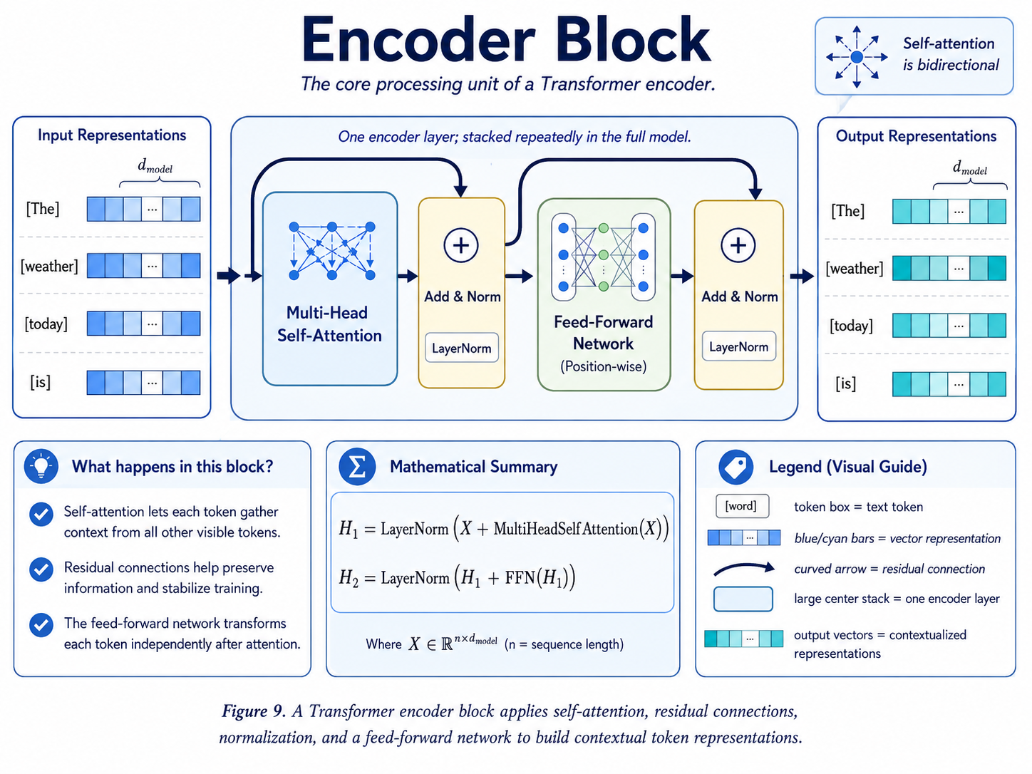
Attention is only one sublayer inside a Transformer block. Its output is wrapped with mechanisms that help deep networks preserve information and train reliably.
5.7.1 Residual connections
A residual connection adds the original input to the sublayer output:
Y = X + \operatorname{Sublayer}(X)
This creates a direct route through the network.
Instead of requiring each layer to reconstruct the entire representation from the beginning, the layer can learn a useful adjustment to the representation it received.
A useful interpretation is:
New representation
=
Existing representation
+
Useful modification
Residual connections improve gradient flow through deep networks and reduce the risk that important information is destroyed by every transformation.
5.7.2 Layer normalization
Layer normalization rescales the features of each token representation using its mean and variance:
\hat{x}
=======

\frac{x-\mu}{\sqrt{\sigma^2+\epsilon}}
A learned scale and bias are then applied:
y=\gamma\hat{x}+\beta
Normalization helps keep activations in a stable numerical range.
5.7.3 Post-normalization and pre-normalization
The original Transformer used a post-normalization arrangement:
\operatorname{LayerNorm}
\left(
X+\operatorname{Sublayer}(X)
\right)
Many later architectures use pre-normalization:
X+\operatorname{Sublayer}
\left(
\operatorname{LayerNorm}(X)
\right)
Research has shown that the location of layer normalization affects gradient behaviour and training stability. Pre-normalization is common in many deep modern Transformer implementations, although specific architectures vary.
5.7.4 Dropout
During training, dropout may randomly suppress selected activations or attention probabilities. This discourages the model from depending excessively on particular pathways and acts as a regularizer.
Dropout is generally disabled during inference.
Step 5.8: The Position-Wise Feed-Forward Network
After attention allows tokens to gather information from one another, each token passes independently through a feed-forward neural network.
The standard form is:
FFN(x)
======

\sigma(xW_1+b_1)W_2+b_2
where (\sigma) is a nonlinear activation such as ReLU, GELU, SwiGLU, or another architecture-specific function.
Typically, the network:
- expands the vector from (d_{\text{model}}) to a larger hidden dimension (d_{\text{ff}});
- applies a nonlinear transformation;
- projects the result back to (d_{\text{model}}).
For example:
768 dimensions
      ↓
3,072 dimensions
      ↓
768 dimensions
Attention mixes information; the feed-forward network transforms it
This distinction is useful:
- Attention moves and combines information among token positions.
- The feed-forward network performs a learned nonlinear transformation at each position.
The same feed-forward weights are applied to every token position, but each token enters with a different contextual representation and therefore produces a different result.
A simple analogy is:
Attention gathers the relevant documents. The feed-forward network reads and processes the resulting file.
The feed-forward sublayer is also enclosed by a residual connection and normalization.
Step 5.9: The Complete Encoder Block
A classical Transformer encoder layer contains:
- multi-head self-attention;
- residual connection and layer normalization;
- position-wise feed-forward network;
- another residual connection and layer normalization.
In simplified post-normalization form:
H_1 =
\operatorname{LayerNorm}
\left(
X+\operatorname{MultiHeadSelfAttention}(X)
\right)
H_2 =
\operatorname{LayerNorm}
\left(
H_1+FFN(H_1)
\right)
The resulting matrix still contains one vector per input token.
Several encoder layers are stacked:
Input representations
        ↓
Encoder layer 1
        ↓
Encoder layer 2
        ↓
Encoder layer 3
        ↓
...
        ↓
Final contextual representations
Early layers may capture relatively local or surface-level patterns, while later layers can construct increasingly abstract task-relevant representations. This should not be interpreted as a rigid hierarchy with perfectly assigned responsibilities; representations are distributed across layers and components.
5.9.1 Encoder-only output
An encoder-only model can use the final representations in several ways:
- classify the entire sequence;
- classify individual tokens;
- identify entities;
- produce embeddings;
- answer extractive questions;
- estimate semantic similarity.
BERT, for example, was designed to learn bidirectional representations by conditioning on both left and right context in its encoder layers.
Step 5.10: The Complete Decoder Block
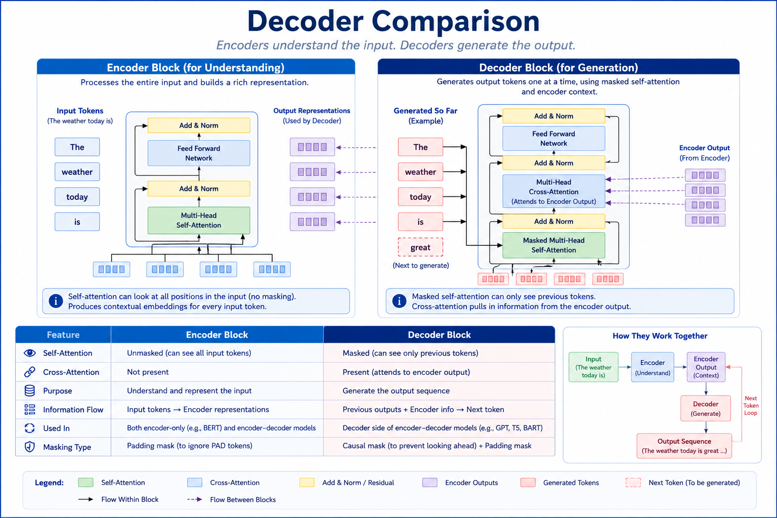
The decoder in the original encoder–decoder Transformer contains three major sublayers:
- masked multi-head self-attention;
- cross-attention over encoder outputs;
- a position-wise feed-forward network.
Each sublayer is accompanied by residual and normalization operations.
5.10.1 Masked self-attention
The decoder first examines the output tokens generated so far. The causal mask prevents it from seeing future target tokens.
5.10.2 Cross-attention
The decoder must also consult the input represented by the encoder.
In cross-attention:
- queries come from the decoder;
- keys come from the encoder output;
- values come from the encoder output.
Symbolically:
Q = H_{\text{decoder}}W_Q
K = H_{\text{encoder}}W_K
V = H_{\text{encoder}}W_V
This lets each decoder position identify which parts of the input are relevant to the output token currently being produced.
For summarization, the decoder may consult the sentence containing the main result. For translation, it may align a target-language token with one or more source-language tokens. For question answering, it may focus on the passage segment containing the answer.
5.10.3 Feed-forward processing
The cross-attention result then passes through the feed-forward sublayer, residual path, and normalization.
5.10.4 Decoder-only models
A decoder-only model removes the separate encoder and cross-attention system. Each block generally contains:
- causal self-attention;
- a feed-forward or gated MLP sublayer;
- residual pathways;
- normalization.
The prompt and generated continuation occupy the same sequence. Every generated token can attend to the prompt and to previously generated tokens, but not to future tokens.
Step 5.11: Output Projection and Softmax
After the final Transformer layer, the model has a contextual vector for every position.
For language generation, the vector at the relevant position is projected into vocabulary-sized logits:
z = hW_{\text{vocab}}+b
If the vocabulary contains 50,000 tokens, the output contains 50,000 logits.
Softmax converts these logits into probabilities:
P(token_i)
==========

\frac{e^{z_i}}
{\sum_j e^{z_j}}
For the sequence:
The spacecraft entered
the model might produce an illustrative distribution such as:
orbit       0.41
the         0.10
Earth's     0.08
a           0.06
safely      0.04
...
A decoding procedure chooses the next token. Depending on the application, this may involve:
- selecting the highest-probability token;
- sampling from the distribution;
- adjusting temperature;
- restricting selection to top-ranked candidates;
- using beam search in sequence-to-sequence tasks.
The chosen token is appended to the sequence, and the process repeats until the model generates a stopping token or reaches another termination condition.
The Transformer does not normally draft an entire paragraph in one indivisible act. It repeatedly predicts a token, adds it to the context, and predicts again. Its apparent fluency emerges from a very large number of individually modest decisions.
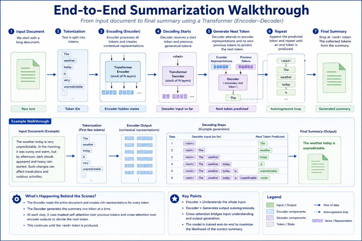
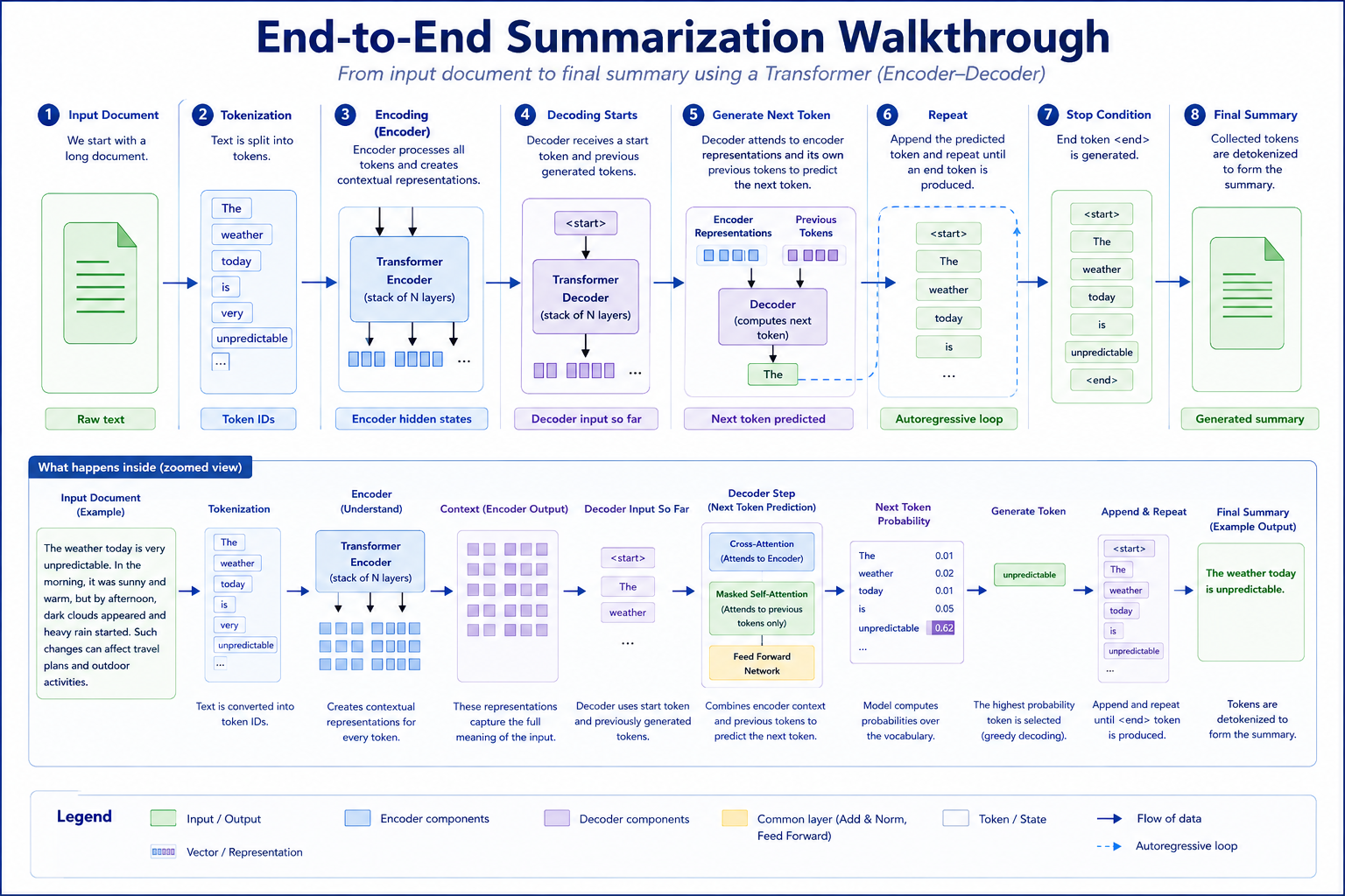
6. An End-to-End Walkthrough
Consider an encoder–decoder model that summarizes:
“The engineering team postponed the software release because a critical authentication defect was discovered during final testing.”
A desired summary might be:
“The release was postponed because of a critical authentication defect.”
Here is how the information travels through the system.
Step 6.1: Tokenization
The input is divided into tokens and mapped to token IDs.
["The", " engineering", " team", " postponed", ...]
Step 6.2: Embedding lookup
Every token ID selects a trainable embedding vector.
The result is an (n \times d_{\text{model}}) matrix.
Step 6.3: Add positional information
Each token representation receives information about its position.
The model can now distinguish:
team postponed release
from:
release postponed team
The second sequence may be grammatically adventurous, but it should not be numerically indistinguishable from the first.
Step 6.4: Encoder self-attention
Every input token creates queries, keys and values.
The token postponed may attend strongly to:
- team as the acting entity;
- release as the affected object;
- because as a causal connector;
- defect as the primary reason.
The token defect may attend to:
- critical;
- authentication;
- discovered;
- testing.
Step 6.5: Encoder multi-head attention
Several heads examine different relationship patterns in parallel.
One head may emphasize causal structure. Another may connect descriptive modifiers. Another may preserve long-range dependency between postponed and defect.
Step 6.6: Encoder residual, normalization and feed-forward processing
The attention output is integrated with the previous representation. The feed-forward network then transforms each contextualized token vector.
Step 6.7: Repeat the encoder layers
The sequence passes through the entire encoder stack. The final output is a contextual representation of the source text.
Step 6.8: Begin the decoder
The decoder receives a start token or an initial target prefix.
Its masked self-attention can inspect only target tokens already available.
Step 6.9: Cross-attention
The decoder queries the encoder representations.
When generating postponed, it may focus on the source tokens postponed and release. When generating authentication defect, it may attend strongly to those source terms while assigning less importance to engineering team or final testing.
Step 6.10: Produce vocabulary probabilities
The decoder’s final hidden representation is projected into vocabulary logits and converted to probabilities.
The model selects or samples the next token.
Step 6.11: Append and repeat
Suppose the partial summary is:
The release was
The decoder predicts the next token, perhaps postponed. The updated sequence becomes:
The release was postponed
The process repeats until the summary is complete.
7. Training a Transformer
The architecture defines how inputs are transformed into outputs. Training determines what the model’s parameters learn to do.
The parameters include:
- token embeddings;
- query, key and value projection matrices;
- output projections;
- feed-forward weights;
- normalization parameters;
- output vocabulary projections;
- positional parameters in architectures that learn them.
Training repeatedly performs:
- a forward pass;
- loss calculation;
- backpropagation;
- parameter updates through an optimizer.
7.1 Causal language modelling
Decoder-only language models are commonly trained to predict the next token.
Given:
The server returned an error
the training examples are conceptually:
Input:  The
Target: server

Input:  The server
Target: returned

Input:  The server returned
Target: an

Input:  The server returned an
Target: error
In practice, causal masking allows predictions for many positions to be calculated in parallel during training.
The objective maximizes:
P(x_t \mid x_1,x_2,\ldots,x_{t-1})
across the training sequence.
7.2 Masked language modelling
Encoder models such as BERT can hide selected tokens and train the model to reconstruct them using context on both sides.
The database rejected the [MASK].
The model may infer request from the surrounding text.
Because the encoder is not causal, it can incorporate both earlier and later tokens.
7.3 Sequence-to-sequence learning
Encoder–decoder models receive an input sequence and a target output sequence.
Possible tasks include:
- translation;
- summarization;
- structured extraction;
- question answering;
- rewriting;
- converting instructions into outputs.
T5 demonstrated how many NLP tasks could be expressed in a unified text-to-text format.
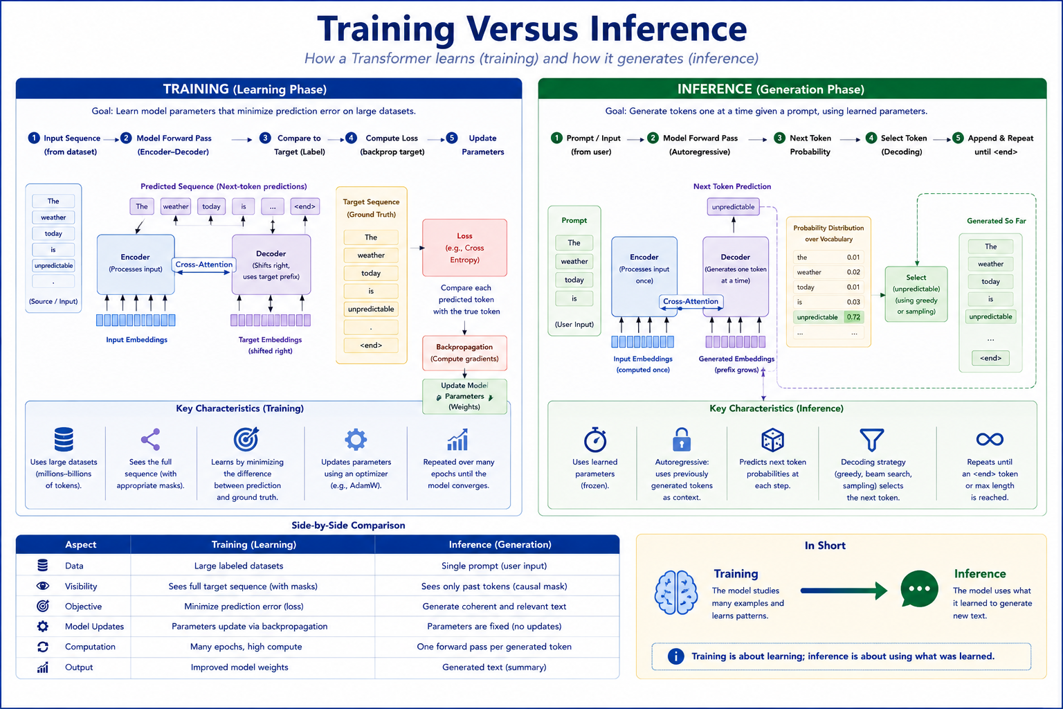
7.4 Teacher forcing
During encoder–decoder training, the decoder is commonly given the correct earlier target tokens while learning to predict the next one.
For target text:
The release was postponed.
the decoder input and prediction targets are shifted:
Decoder input:  <START> The release was postponed
Targets:         The    release was postponed .
Teacher forcing makes training efficient, although inference differs because the model must then condition on its own previously generated outputs.
7.5 Cross-entropy loss
For a correct target token (y_t), the loss can be expressed as:
L_t = -\log P(y_t)
The total training loss averages or sums this quantity across relevant token positions.
If the model assigns high probability to the correct token, the loss is low. If it confidently predicts the wrong token, the loss becomes large. Confidence is useful, but misplaced confidence receives an invoice.
7.6 Backpropagation
Gradients flow backward through:
- the output projection;
- feed-forward layers;
- attention operations;
- embeddings;
- and all stacked Transformer layers.
An optimizer adjusts the parameters to reduce future loss.
This is how the model learns attention patterns. Engineers do not manually specify that it should attend to satellite or that defect should relate to authentication. Training data and the learning objective shape those relationships.
8. Training Versus Inference
The distinction between training and inference resolves an apparent contradiction:
Transformers are highly parallel, yet generative models produce tokens one at a time.
Both statements are true.
8.1 Parallelism during training
When the target sequence is already known, a causal mask allows the model to calculate representations for many positions simultaneously while preventing future-token leakage.
This is a major advantage over recurrent architectures, which generally process sequence states through an inherently sequential dependency chain.
8.2 Autoregressive inference
During generation, future tokens do not yet exist.
The model must:
- process the available sequence;
- predict the next token;
- append it;
- repeat.
TensorFlow’s Transformer tutorial similarly describes autoregressive models as generating text one token at a time and feeding each generated output back into the model.
8.3 Key-value caching
Naively, the model could recompute keys and values for every earlier token at every generation step.
A KV cache stores the key and value tensors from previous positions. The next step then computes new keys and values only for the latest token while reusing the stored tensors.
Conceptually:
Without cache:
Recalculate the entire conversation repeatedly.

With cache:
Remember the earlier calculations and process only the new arrival.
The cache reduces repeated computation but consumes memory that grows with sequence length, number of layers, and key–value dimensions.
9. Why Transformers Work So Well
No single property fully explains the success of Transformers. Their effectiveness emerges from several mutually reinforcing advantages.
9.1 Direct access to context
Self-attention allows one token to interact directly with another visible token, regardless of their distance in the sequence.
In a recurrent model, information from an early token may need to pass through many intermediate states. In self-attention, a distant token can receive a direct connection through the attention matrix.
9.2 Parallel training
Because attention does not depend on a recurrent hidden-state chain, many sequence positions can be processed together during training.
This substantially improves hardware utilization.
9.3 Scalable repetition
The same basic block can be stacked many times:
Attention
→ MLP
→ Attention
→ MLP
→ Attention
→ MLP
...
Depth, width, number of heads, training data and compute can all be increased while retaining a conceptually regular architecture.
9.4 Dynamic context
The contribution of each token is computed from the current input.
The representation of port can adapt depending on whether the surrounding context discusses:
- networking;
- shipping;
- software;
- wine;
- or a physical connector.
9.5 Flexible modality
The architecture mainly needs a sequence or set of input representations.
Those units may be:
- text tokens;
- image patches;
- audio segments;
- video patches;
- biological residues;
- source-code tokens;
- sensor observations;
- combinations of several modalities.
Vision Transformer demonstrated that an image could be divided into patches, embedded as a sequence, and processed using a largely standard Transformer encoder.
10. Transformer Limitations
Transformers are powerful, but their design introduces important costs and constraints.
10.1 Quadratic attention complexity
For (n) tokens, standard self-attention constructs an (n \times n) score matrix.
The number of pairwise relationships therefore grows approximately as:
O(n^2)
Doubling the sequence length can increase the size of the attention matrix by roughly four times.
This makes long contexts computationally and memory intensive.
FlashAttention improves performance by reorganizing exact attention computation to reduce expensive transfers between different levels of GPU memory. It does not simply remove the mathematical relationships; it computes them in a more hardware-aware manner.
10.2 Autoregressive generation is sequential
Training can be parallel across known positions, but generation still requires each new token before the next token can be produced.
This creates latency, particularly for long outputs.
10.3 Context is finite
A Transformer can only directly process information that fits within its supported context and memory limits.
Long-context architectures extend this range, but “fits in the context window” does not automatically mean “will be recalled and used perfectly.”
10.4 Data and compute requirements
Large Transformers may require substantial amounts of:
- training data;
- accelerator time;
- electrical energy;
- distributed infrastructure;
- memory;
- storage;
- evaluation effort.
Architectural simplicity does not imply operational simplicity.
10.5 Statistical prediction is not guaranteed truth
A language model estimates likely outputs given its learned parameters and context. Fluency does not guarantee factual accuracy, sound reasoning, current knowledge, or reliable citation.
The model can generate a sentence that is grammatically confident and factually incorrect. Syntax and truth are, regrettably, not bound by an automatic service-level agreement.
10.6 Attention is not a complete explanation
Attention weights can provide useful information about token interactions, but they should not automatically be treated as a complete causal explanation of a model’s decision.
Model behaviour is distributed across:
- attention heads;
- value vectors;
- feed-forward networks;
- residual streams;
- normalization;
- and many layers.
A bright square on an attention heat map is evidence of a computational relationship, not necessarily a full explanation of the model’s reasoning.
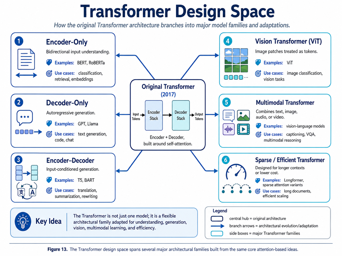
11. Important Transformer Variations
The original architecture has evolved into a broad design family.
11.1 Encoder-only Transformers
Encoder-only models use bidirectional self-attention. Every non-masked token can generally inspect tokens on both sides.
They are well suited to:
- classification;
- semantic embeddings;
- token labelling;
- entity recognition;
- retrieval;
- input understanding.
BERT is the canonical example.
11.2 Decoder-only Transformers
Decoder-only models use causal self-attention.
They are well suited to:
- text generation;
- code generation;
- dialogue;
- continuation;
- instruction-conditioned output;
- tool-call generation.
The same sequence contains both the prompt and the generated continuation.
11.3 Encoder–decoder Transformers
Encoder–decoder models explicitly separate input representation from output generation.
They are especially natural for:
- translation;
- summarization;
- input-conditioned generation;
- structured transformations.
T5 is a prominent example.
11.4 Vision Transformers
A Vision Transformer divides an image into patches:
Image
→ Fixed-size patches
→ Patch embeddings
→ Positional information
→ Transformer encoder
Each patch behaves somewhat like a token. Attention lets image regions exchange information globally.
11.5 Multimodal Transformers
Multimodal systems may represent text, images, audio or video as compatible sequences of embeddings.
Architectural arrangements include:
- separate modality encoders connected through cross-attention;
- unified token streams;
- modality-specific projection layers;
- shared multimodal decoders.
The recurring theme is to convert different information types into representations that attention layers can relate.
11.6 Efficient and sparse attention
To reduce the cost of long sequences, researchers have explored:
- sliding-window attention;
- block-sparse attention;
- local plus global attention;
- low-rank approximations;
- recurrent memory mechanisms;
- retrieval-based context;
- hardware-aware exact attention.
These methods trade among efficiency, memory, implementation complexity and the range of token interactions.
12. A Compact Mathematical Summary
Given an input sequence of (n) token representations:
X \in \mathbb{R}^{n \times d_{\text{model}}}
Create queries, keys and values
Q=XW_Q,\qquad K=XW_K,\qquad V=XW_V
Calculate scaled attention scores
S=\frac{QK^T}{\sqrt{d_k}}+M
Normalize the scores
A=\operatorname{softmax}(S)
Combine value vectors
H=AV
Run multiple attention heads
MHA(X)
======

\operatorname{Concat}(head_1,\ldots,head_h)W_O
Apply residual processing and normalization
In a simplified post-normalization block:
X'=\operatorname{LayerNorm}(X+MHA(X))
Apply the feed-forward network
FFN(X')
=======

\sigma(X'W_1+b_1)W_2+b_2
Apply the second residual path
Y=\operatorname{LayerNorm}(X'+FFN(X'))
The output (Y) becomes the input to the next Transformer layer.
For language generation, the final representation is projected into vocabulary logits:
Z=YW_{\text{vocab}}+b
and converted into token probabilities:
P=\operatorname{softmax}(Z)
That is the core machinery. Modern systems may contain billions of parameters and extensive engineering optimizations, but the architectural foundation remains recognizable within these operations.
13. A Practical Mental Model
When trying to remember the architecture, use the following sequence:
13.1 Represent the input
Tokens → embeddings + positions
13.2 Let tokens exchange information
Queries + keys + values → attention
13.3 Use several perspectives
Multiple attention heads
13.4 Preserve and stabilize information
Residual connections + normalization
13.5 Transform each contextualized token
Feed-forward network
13.6 Repeat the block
More layers → richer representations
13.7 Convert representations into a task output
Classification, embedding or next-token probabilities
Or, in one sentence:
A Transformer repeatedly lets each token gather relevant information from other tokens, transforms the resulting representation, and preserves useful information through residual pathways.
14. Deep Learning Versus Transformer Architecture
The terms deep learning and Transformer architecture are sometimes used as though they describe the same thing. They do not.
Deep learning is the broader field. A Transformer is one particular neural-network architecture developed within that field.
A useful hierarchy is:
Artificial Intelligence
  ↓
Machine Learning
  ↓
Deep Learning
  ↓
Neural-network architectures
  ├── Convolutional Neural Networks
  ├── Recurrent Neural Networks
  ├── Autoencoders
  ├── Graph Neural Networks
  ├── Transformers
  └── Other architectures
In other words, every Transformer model is a deep-learning model, but not every deep-learning model is a Transformer.
A convolutional neural network used to classify medical images is a deep-learning system. An LSTM used to forecast sensor readings is also a deep-learning system. Neither necessarily uses Transformer architecture.
14.1 What deep learning refers to
Deep learning is a branch of machine learning based on neural networks containing multiple successive layers of learned transformations.
The word deep refers primarily to the number of computational layers through which information passes, not to the model possessing unusually profound thoughts, despite what some product demonstrations may imply.
A typical deep-learning system contains:
- trainable parameters such as weights and biases;
- multiple layers of mathematical transformations;
- nonlinear activation functions;
- a loss function that measures prediction error;
- backpropagation to calculate gradients;
- an optimizer that updates the parameters.
Suppose a neural network receives an image of a vehicle. Early layers may respond to edges and colour transitions. Intermediate layers may combine these signals into shapes, textures and components. Later layers may represent more abstract patterns such as wheels, windows or the overall form of a car.
The precise type of processing depends on the architecture, but the general deep-learning principle remains the same:
Information passes through several trainable layers, and the model learns useful internal representations by adjusting its parameters to reduce prediction error.
Deep learning therefore describes a broad method of constructing and training multilayer neural networks. It does not prescribe one specific arrangement of those layers.
14.2 What a Transformer refers to
A Transformer is a particular design for arranging deep-learning components.
Its defining feature is the use of attention mechanisms to model relationships among elements in a sequence. A Transformer commonly includes:
- token or input embeddings;
- positional information;
- query, key and value projections;
- multi-head attention;
- feed-forward neural networks;
- residual connections;
- normalization layers;
- stacked encoder or decoder blocks.
The Transformer is still a neural network. Its attention projections, output projections and feed-forward layers all contain trainable weights. It is trained using the same broader deep-learning machinery: forward passes, loss calculation, backpropagation and optimization.
What makes it a Transformer is not that it uses deep learning, but the specific way its layers allow input elements to exchange information through attention.
For example, in:
The weather today is
each token begins as an embedding. Self-attention allows the representation of is to incorporate information from The, weather and today. Feed-forward layers then transform the resulting contextual representation. After several Transformer layers, the model produces a probability distribution for the next token, perhaps assigning the highest probability to great.
A conventional deep neural network could also process numerical inputs and produce predictions, but it would not necessarily use this query-key-value attention process.
14.3 The relationship between the two
| Deep learning | Transformer architecture |
|---|---|
| A broad branch of machine learning | A specific neural-network architecture |
| Includes many different model families | Belongs to the deep-learning family |
| Defines general learning mechanisms | Defines a particular arrangement of layers |
| Commonly uses backpropagation and gradient-based optimization | Is usually trained using those same methods |
| Includes CNNs, RNNs, LSTMs, autoencoders, Transformers and others | Primarily uses attention, feed-forward layers, residual paths and normalization |
| Can be applied to images, text, audio, graphs and numerical data | Can also process many modalities once they are represented as tokens or vectors |
Deep learning supplies the general learning framework. The Transformer supplies a particular structural blueprint.
An engineering analogy may help:
Deep learning is the discipline of designing and training complex computational machines.
A Transformer is one highly successful machine design within that discipline.
The distinction is similar to the relationship between civil engineering and a suspension bridge. Civil engineering contains the principles, methods and materials used to construct many types of structures. A suspension bridge is one particular architectural solution created using those principles.
14.4 How Transformers differ from earlier deep-learning architectures
Transformers did not replace the fundamental principles of deep learning. They changed how sequence information is processed.
Recurrent neural networks
RNNs and LSTMs process sequences through a recurring hidden state. Information travels from one sequence position to the next:
Token 1 → Token 2 → Token 3 → Token 4
This provides an inherent sense of order, but it also creates sequential computation and can make long-distance dependencies difficult to preserve.
Convolutional neural networks
CNNs use learned filters that examine local neighbourhoods. They are especially effective for images and other data with strong local structure.
A convolution may first identify nearby patterns, while deeper layers gradually expand the effective receptive field.
Transformers
Transformers allow each visible token to communicate more directly with other tokens through attention:
Token 1 ↔ Token 2 ↔ Token 3 ↔ Token 4
The model dynamically calculates which relationships are important for the current input. This makes Transformers particularly effective when dependencies may occur across long distances.
The architectures differ primarily in their inductive biases, the structural assumptions built into how they process information:
- CNNs strongly emphasize local neighbourhoods.
- RNNs strongly emphasize sequential state transitions.
- Transformers strongly emphasize dynamically learned relationships through attention.
None of these assumptions is universally superior. The best architecture depends on the structure of the data, the task, computational constraints and the desired behaviour.
14.5 Is a Transformer the same as a large language model?
No. This is another useful distinction.
A Transformer is an architecture. A large language model is a trained model, usually built using a Transformer architecture, whose parameters have been learned from a large text or multimodal dataset.
The relationship is approximately:
Deep learning
    ↓
Transformer architecture
    ↓
Large Transformer model
    ↓
Pretraining on large datasets
    ↓
Language model or multimodal model
GPT-style models, for example, use decoder-only Transformer architectures. BERT uses an encoder-based Transformer. T5 uses an encoder-decoder Transformer.
However, the architecture alone is not what gives a model its complete capabilities. Those capabilities also depend on:
- the training data;
- the learning objective;
- model size;
- tokenization;
- context length;
- optimization process;
- fine-tuning or instruction tuning;
- reinforcement or preference-learning methods;
- inference and decoding strategies;
- external tools and retrieval systems.
Two models can use broadly similar Transformer blocks yet behave very differently because they were trained with different data, objectives and post-training methods.
14.6 Why Transformers are still called deep networks
Although attention receives most of the architectural publicity, a Transformer remains deep because it stacks many layers.
A simplified decoder-only model may repeatedly apply:
Masked self-attention
  ↓
Residual connection and normalization
  ↓
Feed-forward network
  ↓
Residual connection and normalization
If this block is repeated dozens or hundreds of times, the result is a deep neural network.
Each layer receives the representations produced by the preceding layer and modifies them. The model therefore builds increasingly contextual and task-relevant representations as information travels through the stack.
Attention determines which token information should be combined. Feed-forward networks help determine how the combined information should be transformed. Residual connections preserve useful signals, while normalization contributes to stable computation and training.
The Transformer is therefore not an alternative to deep learning. It is one of deep learning's most influential architectural expressions.
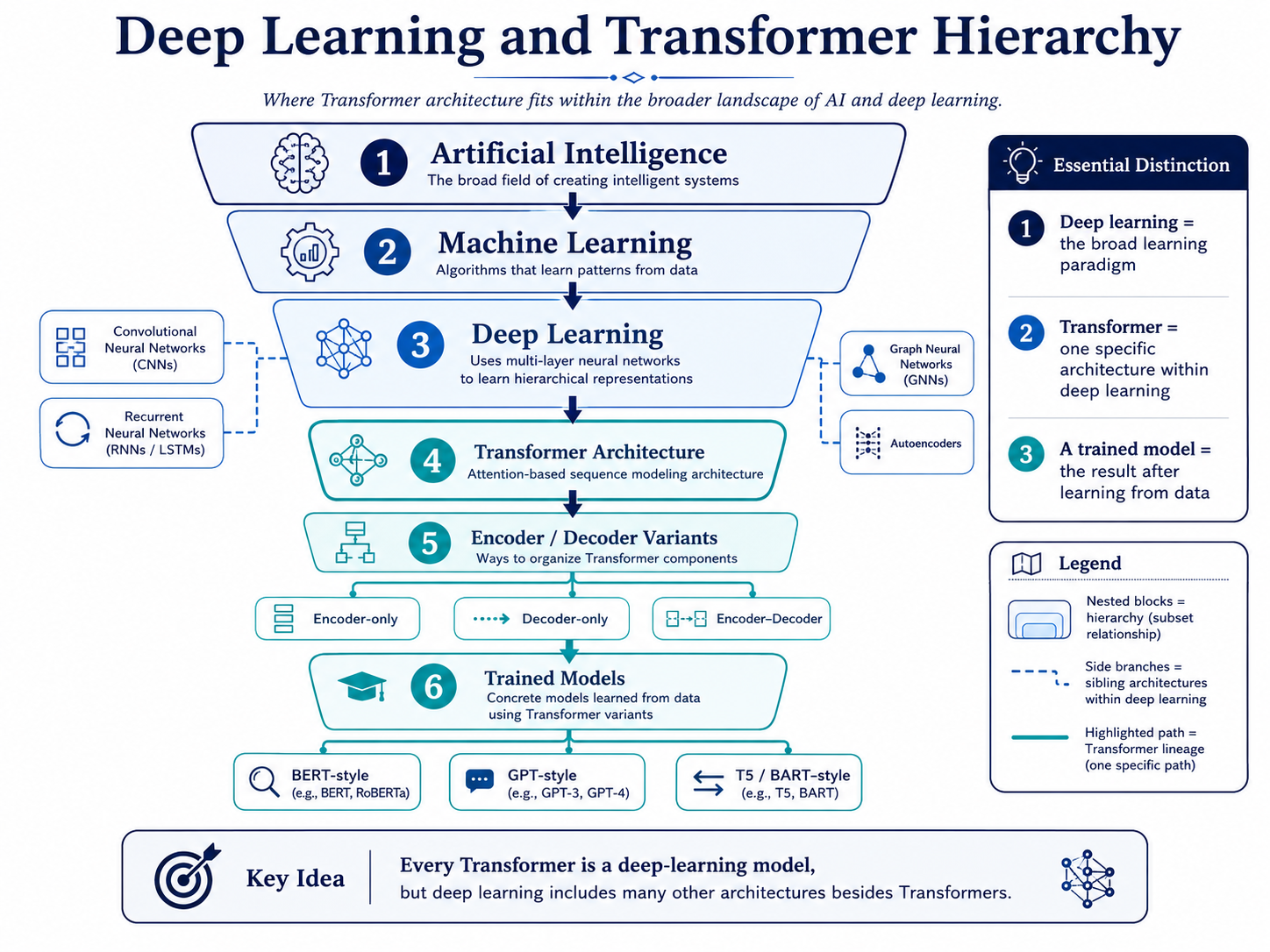
14.7 The essential distinction
The difference can ultimately be remembered in one sentence:
Deep learning describes the broader method of learning through multilayer neural networks; a Transformer describes one specific attention-based architecture used to construct such a network.
Understanding this distinction helps separate three ideas that are often blended together:
Deep learning       = the broader learning paradigm
Transformer         = the architectural blueprint
A trained model     = the resulting system after learning from data
The architecture defines how information can flow. Training determines the parameter values that shape that flow. The resulting model behaviour emerges from both.
15. Conclusion
The Transformer changed deep learning not by introducing one mysterious operation, but by reorganizing sequence modelling around a powerful principle: relationships among elements should be learned dynamically through attention rather than carried exclusively through a sequential recurrent state.
Its process can be summarized as follows:
- input is divided into tokens or other representable units;
- each unit becomes an embedding;
- positional information preserves order;
- queries, keys and values calculate contextual relevance;
- multi-head attention examines several relationship spaces;
- residual connections and normalization stabilize deep processing;
- feed-forward networks transform each contextual representation;
- stacked blocks progressively construct richer representations;
- output layers convert those representations into predictions.
The original architecture combined an encoder and decoder for translation. Subsequent models showed that its components could be rearranged for understanding, generation, vision, multimodal learning and many other tasks.
Transformers are therefore best understood not as one fixed model, but as a reusable architectural language: a collection of components that lets machines learn which pieces of information should communicate, what they should exchange, and how those exchanges should shape the final prediction.
The mathematics is compact. The learned behaviour is not. That gap between simple repeated operations and remarkably complex emergent capability is precisely what makes the Transformer one of the most consequential architectures in modern deep learning.
References and Further Reading
-
Vaswani, A. et al. (2017). Attention Is All You Need.
-
Sutskever, I., Vinyals, O. and Le, Q. V. (2014). Sequence to Sequence Learning with Neural Networks.
-
Bahdanau, D., Cho, K. and Bengio, Y. (2014). Neural Machine Translation by Jointly Learning to Align and Translate.
-
Radford, A. et al. (2018). Improving Language Understanding by Generative Pre-Training.
-
Devlin, J. et al. (2018). BERT: Pre-training of Deep Bidirectional Transformers for Language Understanding.
-
Raffel, C. et al. (2019). Exploring the Limits of Transfer Learning with a Unified Text-to-Text Transformer.
-
Dosovitskiy, A. et al. (2020). An Image Is Worth 16×16 Words: Transformers for Image Recognition at Scale.
-
Kudo, T. and Richardson, J. (2018). SentencePiece: A Simple and Language Independent Subword Tokenizer and Detokenizer.
-
Su, J. et al. (2021). RoFormer: Enhanced Transformer with Rotary Position Embedding.
-
Xiong, R. et al. (2020). On Layer Normalization in the Transformer Architecture.
-
Dao, T. et al. (2022). FlashAttention: Fast and Memory-Efficient Exact Attention with IO-Awareness.
-
PyTorch Documentation. Scaled Dot-Product Attention.
-
PyTorch Tutorials. Implementing High-Performance Transformers with Scaled Dot-Product Attention.
-
TensorFlow Tutorials. Neural Machine Translation with a Transformer and Keras.
-
Hugging Face Course. Transformer Architectures.
-
Google Machine Learning Crash Course. Transformers and Self-Attention.
-
Amanatulla. Transformer Architecture Explained.